ML ALGORITHMS: The Behind-The-Scenes Series
LINEAR REGRESSION ALGORITHM


LINEAR REGRESSION
Linear regression is a regression-based supervised machine learning algorithm. When the target variable is a continuous real number, this algorithm is used. Linear regression is one of the most basic and widely used Machine Learning algorithms. It is a statistical method for performing predictive analysis. Linear regression models are classified as follows:
- UNIVARIATE LINEAR REGRESSION - examines the relationship between one independent (explanatory variable) variable and one dependent variable.
- MULTIVARIATE LINEAR REGRESSION - is a supervised machine learning algorithm that analyzes multiple data variables.
Linear Regression forecasts continuous/real or numeric variables such as sales, salary, age, product price, and so on. It uses the best line of fit to establish the relationship between the target variable (y) and one or more input variables.
As a result, this regression technique determines a linear relationship between x (input) and y (output). Hence, the name Linear Regression was chosen. This algorithm employs the principles of Ordinary Least Squares (OLS) and Mean Square Error (MSE).
OLS minimizes the sum of squared differences between observed target variables in the data set and observed target variables predicted by the algorithm to estimate the unknown parameters of a linear function.
To achieve the goal of this blog series, I would perform some in-depth analyses of the algorithm, focusing on the UNIVARIATE problem. This would make it easier for me and you to explain and understand concepts.
INTUITION
Every machine learning project aims to improve prediction accuracy based on previous data while minimizing errors from model training and prediction. A linear regression model must go through three critical stages to achieve high accuracy while minimizing loss.
To begin learning, the model makes an initial hypothetical assumption about the values of weight and bias.
It then thrives to find the accuracy of the hypothesis function using an algorithm called Cost Function or Mean Squared Error after adding these assumptions to our linear regression function (in statistics).
However, because the final goal of the linear regression model is to find the weight and bias combination that minimizes the cost function, we employ an algorithm known as Gradient Descent. This algorithm simply updates the parameters to move them to the cost function's global minimum value.
This is roughly how the linear regression model works behind the scenes. Let us now deconstruct each step and see how it all comes together.
BEHIND-THE-SCENE OPERATIONS OF THE LINEAR REGRESSION ALGORITHM
- STAGE 1 (Hypothetical Assumptions) – The linear regression model is mathematically expressed as:
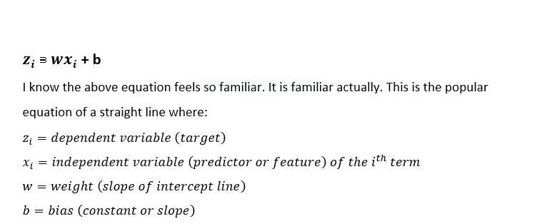 fig1: equation of a straight line aka: Linear Regression Formula
Assume we are given a dataset containing feature x and target y to work with. If we plot our data points on an x-y axis graph, we get:
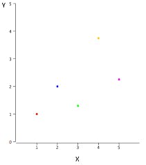 fig2: data points plotted on an x-y plot
The goal is to fit a line - The Most Accurate Line - that passes through almost all of the data points.
The idea behind this first step is to use assumed values for weight and bias as our initial function. Assuming our initial weight and bias values are both 1, and our graph looks like this:
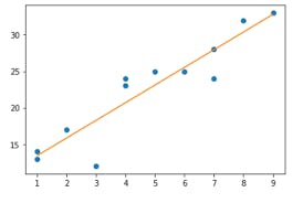 fig3: assumed line of best fit for initial hypothetical assumption.
Our function is now z_i=1x+1. This is referred to as a hypothesis function. Our hypothesis function now appears to be fairly accurate. We use a function called The Cost Function or Mean Squared Error to calculate the function's accuracy. This leads us to the next stage.
- STAGE 2 (Cost Function) – During step 1, the cost function computes the differences between the actual and predicted targets for each data point (hypothetical assumption). The graph below will help us understand this step in greater depth:
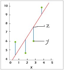 fig4: graph showing prediction error after hypothetical assumption.
Our differences are represented by the lines connecting our hypothesis function (z) and the data points (y). To calculate the average of the sum of errors, we add the sum of the squares of these errors and divide it by the number of data points. The error for a single (x, y) data point is given as:
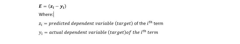 fig5: formula for error of a single data entry (x,y).
We are squaring the difference between the prediction and the actual value because there could be both a -ve and a +ve difference. Because we don't want the sum of these values to be zero, we square the difference to make non positive values positive.
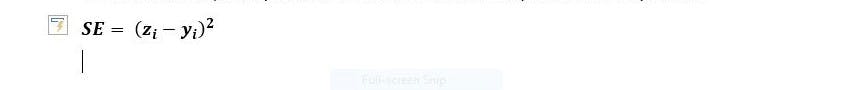 fig6: formula of squared error.
For all data points, the mean of squared error (SE) must be gotten:
 fig7: formula of MSE.
This is the formula for the mean squared error.
Recall that z_i = wx_i + b – therefore, MSE can be rewritten as:
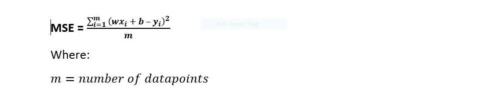 fig8: final MSE formula.
There final cost function (J) is therefore given as:
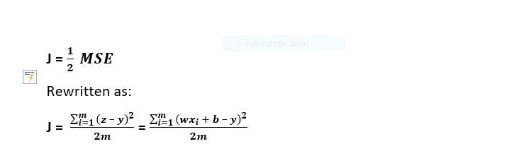 fig9: cost function formula.
- STAGE 3 (Gradient Descent) – The graph of the cost function versus our parameters (w & b) is as follows:
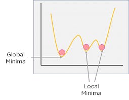 fig10: visual representation of a gradient descent.
Global Minima is the point at which the overall cost is the lowest while the local minima are points other than global minima. Because the goal is to find a pair of parameters (w, b) that minimizes the average error (to global minima - as shown in the diagram above) while still making the most accurate predictions, the linear regression model declares a random vertex or local minima to begin training with and progresses downward as it learns and improves.
We use Gradient Descent to get a parameter to its global minimum point. This algorithm simply updates the weight and bias parameters using the back propagation technique. It computes the next point iteratively using the gradient at the current position, scales it (by a learning rate), and subtracts the obtained value from the current position (makes a step).
This algorithm's steps include: setting up random weights, calculating the slope of the weights point tangent line (derivative), and adjusting parameters until the current slope is 0 or close to it. The gradient descent formula for both the weight and bias parameters is as follows:
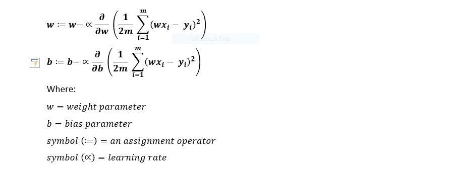 fig11: gradient descent formula for both weight and bias parameters.
PARTS OF THE GRADIENT DESCENT ALGORITHM
- The Assignment Operator (: =) is used to update the weight and bias parameters based on the results of computation during training. This update is necessary so that the cost function can continue to move downwards towards global minima.
- Learning Rate (∝) - controls how the cost function parameters move in search of global minima. Typically, the value of the learning rate ranges between 0.001 and 0.9. Learning rates can be outside of this range, but we want to avoid exceedingly high learning rates, which can cause parameters to miss global minima. We also want to avoid having a low learning rate because this can cause learning to be too slow and lengthy. The best learning rates are obtained by constantly experimenting with values within the conventional range.
- Partial Derivative - In calculus, the partial derivative is simply the 3D version of ordinary derivatives, and it is also used to calculate the slope of a function with respect to a parameter. To determine how each individual parameter affects MSE, we use partial derivatives. These derivatives with respect to w and b are taken separately. With regard to w, this means that we derive parameter w while ignoring what is going on with b, or we can say it is 0 and vice versa. A chain rule will be used to take partial derivatives. We use it to take the derivative of a function that contains another function. According to the chain rule, we should take the derivative of an outside function, leave an inside function alone, and multiply everything by the derivative of the inside function. Therefore, all that remains is to take a partial derivative of the cost function we established earlier with respect to w and b. According to the illustration so far, the learning rate governs the learning steps toward global minima. The steps become much smaller as the slope of the tangent line at the given parameter-point decreases. As a result, we can declare convergence for the parameter when the change in ‘step' is less than a certain threshold value, such as 0.5. We now have the 'perfect' parameters that best fit our data after running the gradient descent for all parameters and declaring convergence.
CONCLUSION
Linear regression algorithm is the most basic machine learning algorithm out here. There is no escaping it either for data science newbies or experts. It is often said that knowing how to use ml algorithms, their parameters and how to evaluate them is all we need. But I argue that a real machine learning engineer must understand the working process of models. Knowing more in depth about a model before use would give an edge while working.
Click the link below to access my code section of this project which I have uploaded in my github. VIEW GITHUB REPO
I would appreciate any form of engagement and correction that could help me improve in my content. I can not wait to see what Machine Learning algorithm I talk about next. We see in two weeks.
REFERENCE LIST
GeeksforGeeks. (2018). ML | Linear Regression. [online] Available at: geeksforgeeks.org/ml-linear-regression/#:~:...
Hurturk, E. (2021). The intuition of Univariate Linear Regression. [online] Medium. Available at: ehurturk.medium.com/intuition-of-univariate.. [Accessed 15 Jul. 2022].
Turin, A. (2020). Gradient Descent From Scratch. [online] Medium. Available at: towardsdatascience.com/gradient-descent-fro...
javatpoint.com. (n.d.). Linear Regression in Machine learning - Javatpoint. [online] Available at: javatpoint.com/linear-regression-in-machine...
keystagewiki.com. (n.d.). Line of Best Fit - Key Stage Wiki. [online] Available at: keystagewiki.com/index.php/Line_of_Best_Fit [Accessed 13 Jul. 2022]equation of a strIg